Control of Virtual and Real Manufacturing Systems in AR/VR
Shanghai Jiao Tong University Capstone Design
Introduction
Imagine in this pandemic of Covid-19, some engineers have no access to manufacturing machines. Or, imagine we students want to learn to use some machines in the factory. How can we learn this online? So our motivation is to use virtual reality and augmented reality technology to synchronously show the manufacturing process and simulate the milling process.
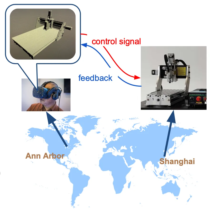
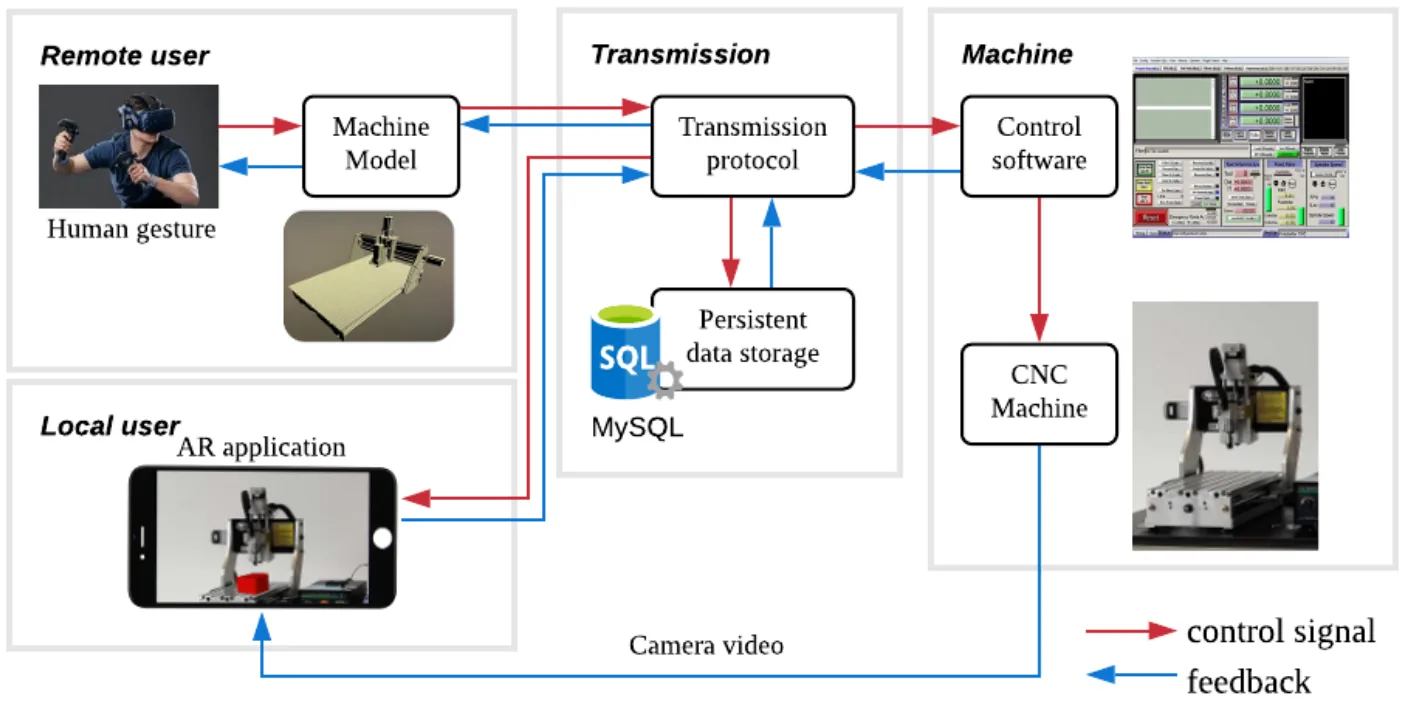
Before heading to the details, we first have a overview of our system. There are three main parts: user, transmission and machine. The remote users could control the machine by gesture and observe the machine with VR headset. The local user can use the mobile application to see a virtual workpiece rendered on the screen. The red arrow represents control signals input; while blue arrows are real-time feedbacks from the machine. Our system looks complicated at first sight, but it would be clear later.
Requirements and Concept Generation
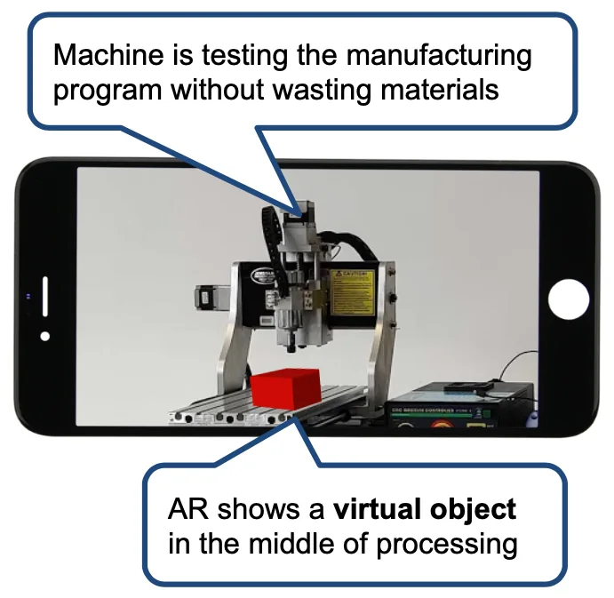
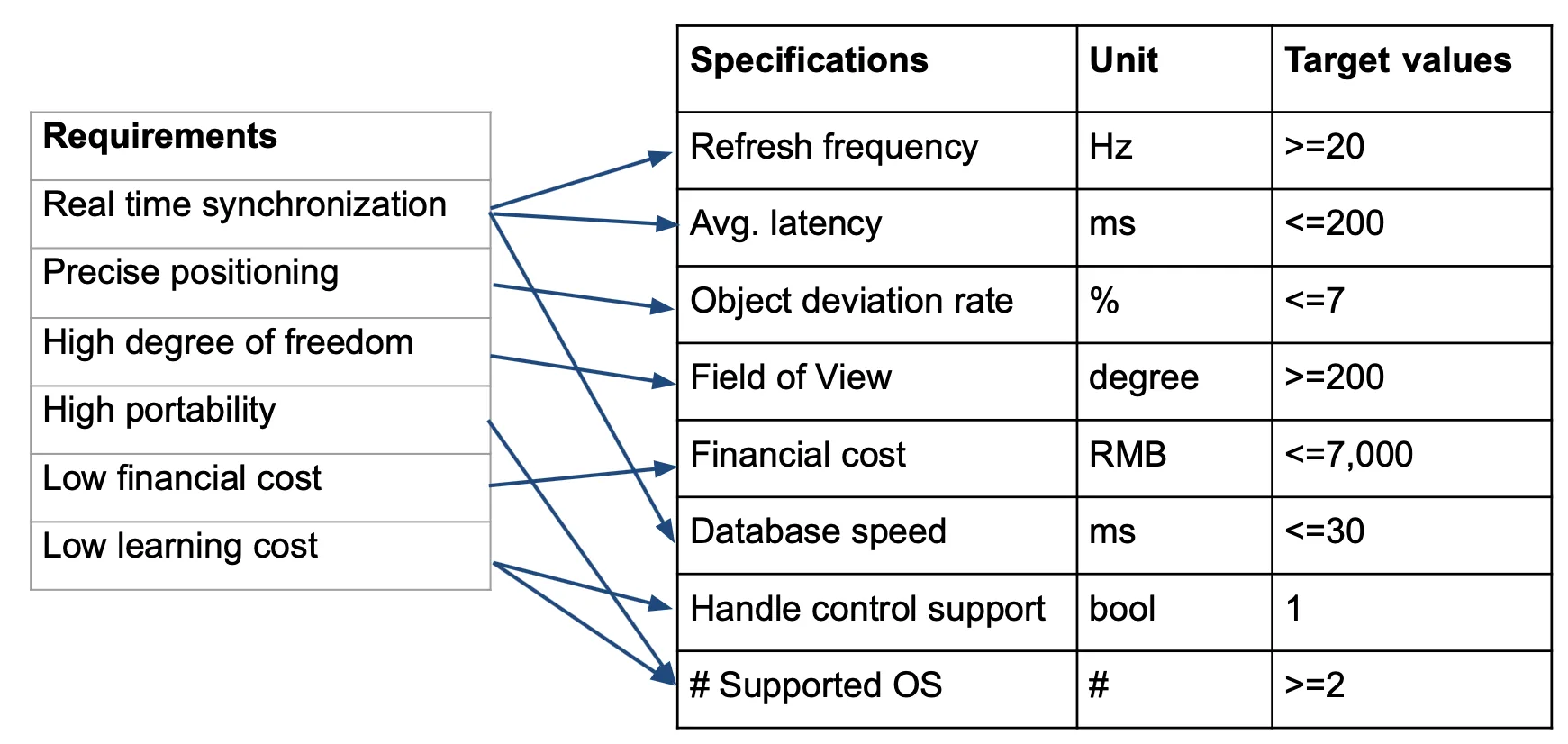
In terms of needs, for VR part, users require real time synchronization, high degree of freedom, and immersive experience. For AR part, we need precisely positioning and carving. Particularly, a sample of AR effect is shown here. Users will scan the machine without materials to know how an artifact will be manufactured. It helps validate the correctness of manufacturing program without wasting materials. For both subfunctions, users need high portability, low financial cost and low learning cost.
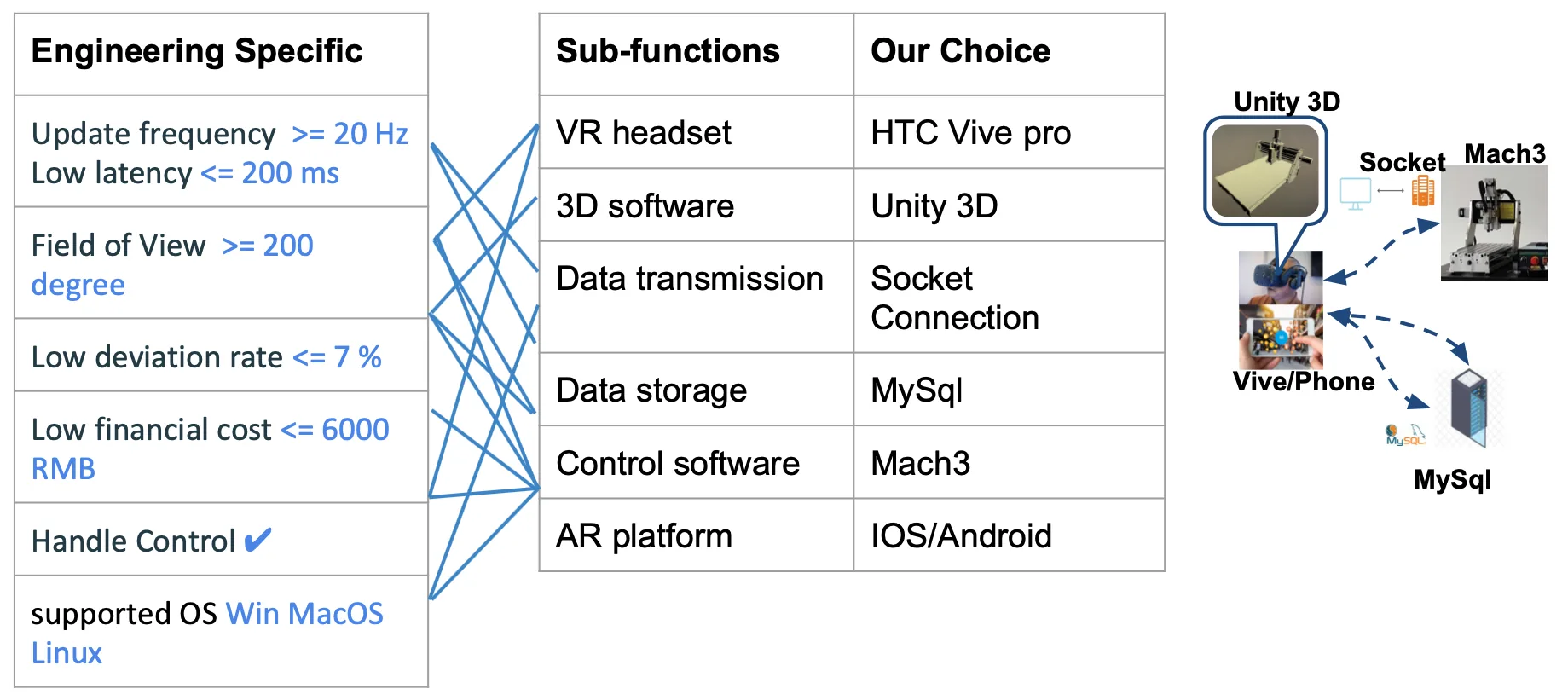
From the needs, we formulate some engineering specifications. We set refresh frequency and latency as the real time criteria and we also add the specifications for object deviation rate, financial cost and so on. The engineering specifications will affect our concept generation and selection.
From the needs, we list out the necessary sub-functions we want to have and choose. We use weight matrices to carry out decision selection based on the engineering specifications. For the user side, we choose HTC Vive Pro as the headset for VR since it a commonly used VR headset with friendly handles and good user experience. We choose smartphones to be the AR terminal because that everyone can download an APP and access to the system. Unity 3D is chose to build the model since it can make and simulate vivid 3D model. For the transmission side, we choose socket connection to reduce the latency and raise the update frequency. Mysql is a stable and fast database that can transmit and store structured data in a short time. For the machine side, we choose Mach3 to control the CNC milling machine, the software can read the real time milling machine status in a low latency.
Design Description
VR System
Now let’s discuss about implementation details. For VR control system part, currently we have implemented environment to enable user to control CNC machine manually to start, move and stop virtually. Also, user may choose to load precompiled Gcode Program to show simulation result of a model. We use Unity Package SteamVR and VRTK to build up the VR environment. Then we setup the control panel by Csharp scripts in Unity which sends user’s commands to MySQL database while simulating CNC machine with data feedback from database.
Real-time Simulation
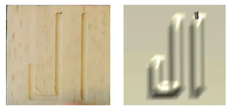
For real-time simulation, we create a brand new algorithm with several Csharp scripts to simulate real time cutting effect of CNC machine in Unity. Below displays actual effect of two controlling methods. In Unity, the program would first generate enough mesh vertices on surface of the piece. Then, whenever the cutter contacts with the vertices, the vertices will modify its height to display cutting effect. This algorithm ensures real-time connection between devices.
AR System
Most parts of the AR environment is a migration from VR. Besides, we utilize vuforia tools to build the AR visualization. We designed the image target to stable the model, which we’ll show later in the demo. Also, we seperate the 3D calculation and the AR visualization to make the whole program run smoothly.
Prototype
VR System
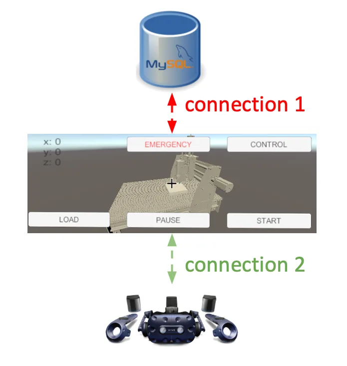
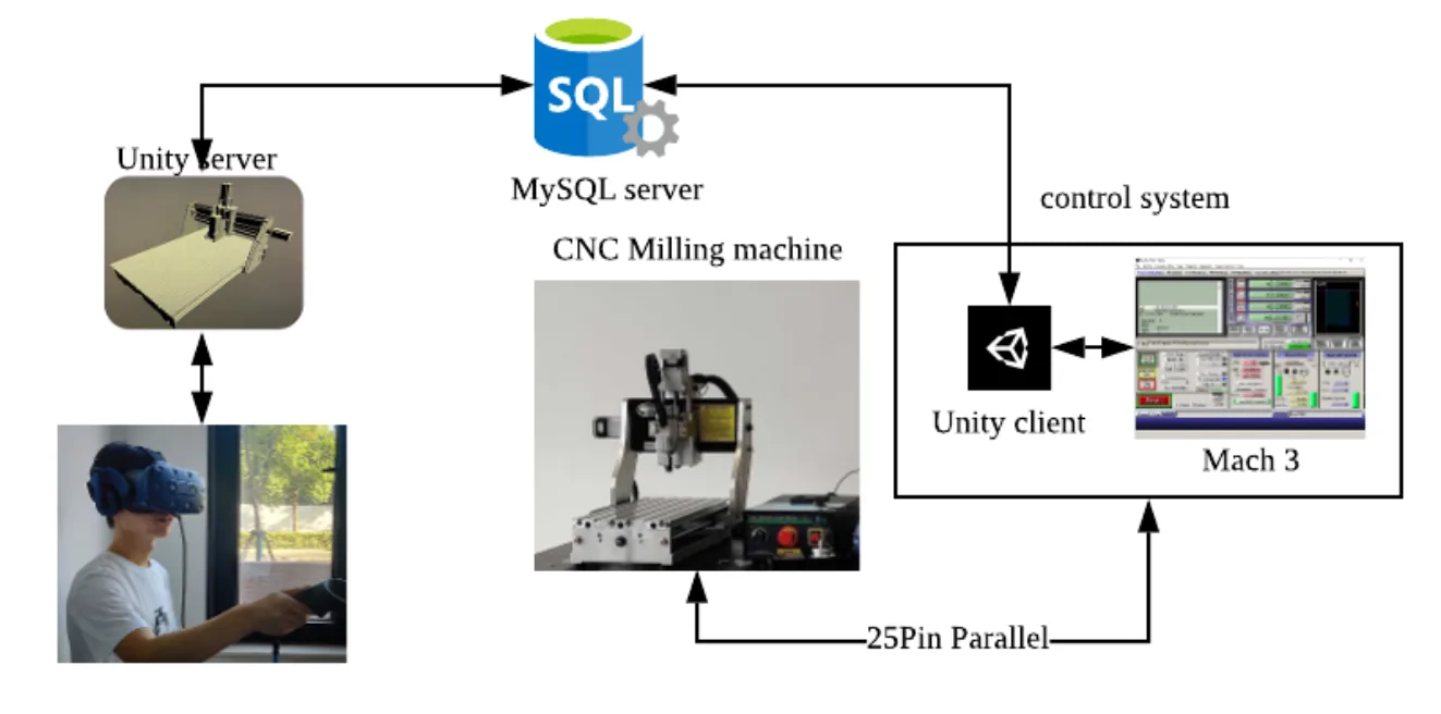
The VR system is built up by three parts: from left to right, remote client, MySQL server and Mach3 client. In the remote client, we built a unity model which is divided into four parts: the base and x, y, z axis. The scale of the coordinate and the directions of the axis are consistent with the real machine. Therefore, given the real-world coordinate, the model will visualize the machine correctly. The Mach3 client is a relay between MySQL server and Mach3. It receives commands from sql and sends to Mach3 and also receives coordinates from Mach3 and sends to sql. MySQL then is a data storage for remote communication. The desktop running Mach3 and Mach3 client is connected to the real machine to operate.
Real-time Simulation
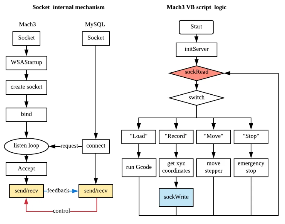
For the real-time transmission, we have two parts. First, the Mach3 client will create connection to the MySQL database and query the data in every loop, which is more than 30Hz, so that once there’s new command (such as “Load” or “Stop”) sent to the database, the client can get it immediately. The second part is the socket transmission. Once the client queries the new command data, it will send it through the socket channel to Mach3. In the meantime, Mach3 VB script will always listen to the socket port, and if there’s any data in the socket channel buffer, it will run sockRead to get the command. With our prototype, the whole transmission process is in real-time.
AR System
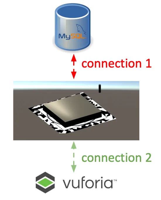
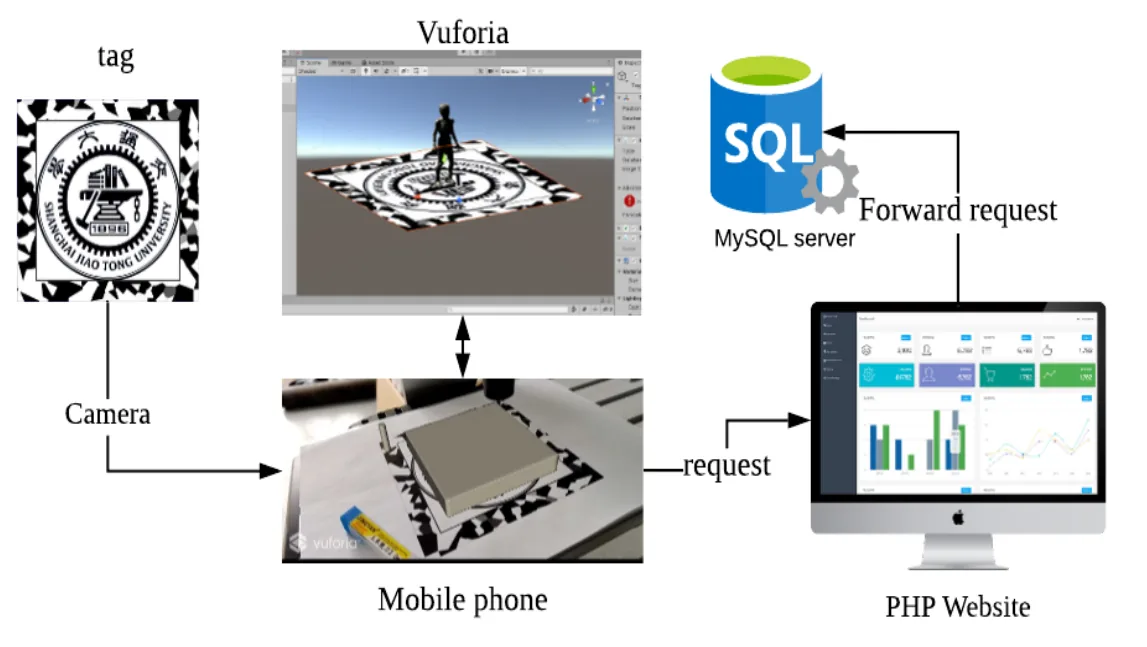
For the AR, the visualization is similar to VR, but it has a different database connection method and a new tag recognition task. Due to mobile security issue, both android and ios don’t allow direct connection to online database. So we wrote a php website on the google cloud platform app engine. It directly connects to the database and opens a web api which is a query to the position data so that on the mobile platform, our program can utilize webrequest package to request the api url to get the data through html form. About the tag recognition, we designed a tag which has a lot of geometric features. The round SJTU logo can help locate the center and the color blocks on the margin have character points which help Vuforia engine determine the direction.
Results
VR Demo
In the video, the right-hand-side is the laptop running our VR model, and on the left is the real cutting process. We can click buttons or use VR device to remote control Mach3 client which is connected to the real physical machine. And the Mach3 client will send back position and moving information back to VR model for visualization. We can see the latency is very low, and it is due to the internet connection and low computing power of the old lab desktop.
AR Demo
Here is the AR APP running on the iOS platform. We can either pre-load our JI cutting model into database or run the Gcode in real-time, and the AR APP can visualize it.
Discussion and Conclusions
Quantitative experiments
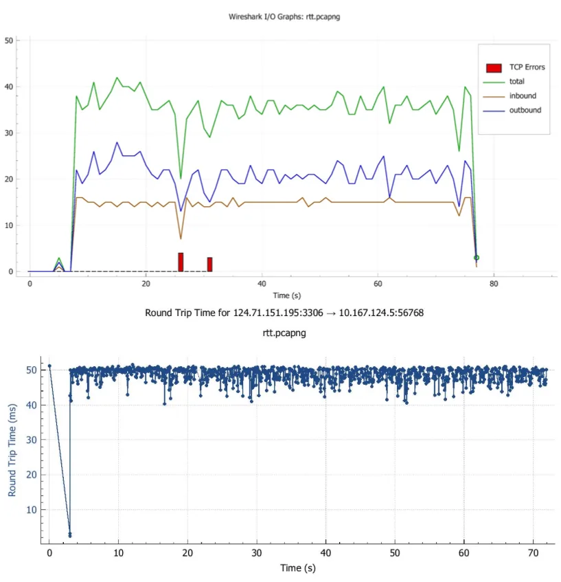
After finishing the prototype, we conducted some experiments for validation. Using the network tool Wireshark, we calculated the frequency of the position feedback, which is around 20 packets per second. At the same time, on the RHS the round-trip time graph shows that the latency is around 50ms, which is lower than our expectation 200ms.
Pros and Cons
Our system enables remote and real-time simulation. Those who are thousands miles away from the machine can still have access to the control and feedback. The database storage enables the users to recap their Gcode programs. However, due to the hardware setting limit, our computer cannot afford greater amount of calculations for higher precision. If we need to simulate a sophisticated artifact, our current design may not give precise enough outcomes.
What-if
Reviewing our design, we found many aspects that we could’ve done better. The first point is computer hardware. Since our CNC Milling machine can only support Windows 7 32bit, it later became our performance bottleneck. If we could start over, we should pay more attention to the choice of hardware. Also, we expect that in the future, AR can adapt itself to the nested mobile device.
Conclusions
In summary, we are dedicated to a remote, real-time control system. Our design used socket connection and MySQL database to record position parameters. We also designed a new shader algorithm for workpiece simulation. In general, our design meets most of the requirements. The server establishment and shader algorithm are the two most important achievements. During this pandemic, we witnessed the power of remote teamwork, and the importance of time management. We are excited and grateful to be a part of this wonderful journey.